Test Apparatus
We will cover tester theory, design, and construction exhaustively in another treatise. Our purpose here is to learn the test procedure, so we will limit our discussion of tester features to essentials. Our test apparatus is comprised of two basic functional components: (1) A mounting platform stage providing linear, translational motion in X and Y axes; and: (2) A very minute light source and knife-edge carried on this stage in a plane perpendicular to our mirror's optical axis.
The knife-edge and the light source are both mounted congruently in a plane (mounted in the same plane) through which the mirror's OA passes perpendicularly. This assembly is in turn mounted on the moveable platform stage so that it can be moved at right angles to and also along (parallel to) the mirror's OA. A dial or screw micrometer is provided for reading the amount of travel of the Y movement stage (motion along or parallel to the OA). Inasmuch as our light source and knife-edge are both mounted on the same plate carried on the platform stage (moving source tester), they move together as a unit in both X and Y axes. Special note: most experienced workers are more familiar with testers having a stationary light source, with only the KE moveable. In our treatise on testers, we will show why carrying both KE and light source together is more advantageous.
Surveying and Measuring the Paraboloid
Figure 8a through 8f shows the appearance of a fully parabolized short focal length mirror for six different positions along its OA as viewed with the KE. By convention we will always begin by pre-setting the micrometer for our tester's Y-axis movement at zero after locating the tester to null the central region of the mirror. From there we will work the KE backwards along the OA away from the mirror, to find the null point, successively, for several different designated zones on the mirror. Below each depiction of the mirror's appearance ("apparition") for each setting of the KE, we show a drawing depicting the mirror's apparent cross-section. Remember, we said we would always think of a concave spherical mirror as flat when viewed as nulled from its center of curvature. Similarly, we will think of the shape of the paraboloid when viewed with the KE as a variation from the flatness of our "flat" reference sphere.
After nulling the very central region of the mirror, we advance the KE away from the mirror and stop at the location shown at fig. 8b. Note that the mirror appears to have an annular, circular "crest" surmounting an apparent, gentle bulge all around its center just a little ways out. Our KE is exactly at the C of C of a very narrow zone surmounting this crest. More accurately (as no zone on a paraboloid can truly have a center of curvature) we are at that point on the OA where that zone's rays are exactly crossing it. Our micrometer will show us, when we inspect it, how far the KE moved backwards to provide this particular apparition of the mirror. The micrometer indicator will show us the KE's location along the OA where this zone's light rays cross over it, relative to its previous location.
We may continue backing the KE away from the mirror, noting, in succession, the other apparitions at c,d,e, and f. The micrometer will always show us the relative location along the OA for the C of C of the narrow zone represented by the crest of the bulge. In addition to being able to locate the C of C for any zone being nulled by our tester fairly precisely along the OA, we can also measure the location of the zone itself on the mirror, its radius from the center of the mirror. And these are the only two quantities we need to determine accurately during the figuring of our mirror in order to shape it into a section of the true paraboloid!
We will pre-determine which zones' centers of curvature we want to monitor before we begin figuring. Conventions or rules about the number and locations of zones for testing vary with workers. The popular convention of dividing the mirror into zones of equal area probably is most advantageous. Zones of equal area will provide for increasingly narrower and more closely bunched zones, successively, outwards towards the mirror's edge. This seems reasonable in that we must figure the outer zones to tighter tolerances than the inner zones. It is very much true, as an older master once told me, that: "The edge zone sets the mirror's performance."
Let us take for an example a project to figure a ten-inch mirror of sixty inches' focal length. To find the location of the middle of each zone (as a radius from the center of the mirror) for any diameter mirror, multiply the mirror's radius (in this case, 5 inches) successively by: 0.316; 0.548; 0.707; 0.837; and 0.945. For our ten inch mirror the middle of each zone computed in this way will, be, successively: 1.58"; 2.74"; 3.53"; 4.185"; and 4.725" as measured from the mirror's center (i.e., as radii).
For the mirror's curve to be the correct section of a true paraboloid for its given diameter and focal length, the C of C of each zone is fixed by formula. The location of each zone's C of C is farther away from the C of C of the very central region of the mirror by the following distances:
| Zone 1 | (1.58"r) | 0.01" |
| Zone 2 | (2.74"r) | 0.031" |
| Zone 3 | (3.53"r) | 0.052" |
| Zone 4 | (4.18"r) | 0.073" |
| Zone 5 | (4.72"r) | 0.093" |
These values are determined by formula (fig. A) where "r" represents the radius of a zone on the mirror and "R" represents the radius of curvature of the mirror (as imagined, of course, as spherical, before figuring). This is not quite the formula most experienced workers are familiar with, as more commonly their testers have their light source fixed and only move the knife edge along the mirror's OA. As we explained previously, we will carry both the KE and the light source on a small plate together in order that we may move them simultaneously along the OA.
It is singular and curious how some obsolete practices continue to be popular very long after much improved ones have been demonstrated. In our article on tester design and construction, we will show several enormous advantages for carrying both KE and light source together, mounted in a specific way.
Locating the Mirror's Zones
We need a practical method for accurately locating any given zone on the mirror for nulling with the tester's knife-edge. Let's look at figure 8d again. This illustration depicts the number three zone (3.53"r) being nulled by our tester's knife edge. This zone divides the mirror into two equal areas, and is by convention referred to as the ".707 zone". How can we be sure that the area being nulled (equally gray all the way around- the gray "crest" of the bulge) is actually centered on the 3.53"r zone? We will put a specially prepared marker in front of the mirror for locating its zones.
Zonal Masks, or Screens
Zone locating masks for Foucault testing are of two basic types. The traditional type has two equal sized apertures cut into the mask for the left and right side of each zone. Over the years I evolved some major improvements in their design and application that improved their accuracy and convenience in use. Finally, though, I discovered the advantages of the "Everest" style zone locating mask, and began to make and use this type exclusively, rapidly incorporating improvements in Everest's basic concept just as I had with the traditional zone locating masks.
Everest's basic approach was to hang a section of yardstick in front of the mirror being tested with pairs of straight pins protruding from one edge to mark the radii of zones for testing. The straight pins would be seen in sharp silhouette against the zone being nulled- one could see their outlines, each on either side of the mirror, against the crest of the "doughnut" behind them. As embodied by Everest, the test is somewhat hampered by a perceptual defect. I have noted this defect and have improved the design by making each pair of straight, vertically standing markers (Everest's "pins") into markers curved to the same radii as the zones they represent. The improvement in certainty when locating a zone with this kind of mask is dramatic.
An example of this kind of mask is shown in figure 9. In this particular example (an early form of my improved design) the little marker "horns" protrude up from the crosspiece that supports them. This earlier example has the pointed tips of the indicator horns lying along a meridian across the mirror's horizontal diameter. Horns about twice as long as these, extending equally above and below the mirror's meridian of horizontal diameter, are even better. These curved indicator horns can be made quite long, since they accurately locate a zone lying everywhere underneath each horn's entire length. A curious perceptual effect is at work here. The longer the horns, the more certain the impression of the crest's location underneath them is. When you make your first zone locating masks, make these horns as long as you please, but each of them must be curved along its entire length to the radius of the zone it is intended to mark.
The mask is easily prepared with a beam compass on poster or illustration board, and then cut out with a sharp hobby knife. The configuration shown in figure 9 is just about perfect - but extend the narrow, curved horns upwards through the mirror's middle, horizontal diameter farther than I show them. I have gotten best results with masks that have the horns extending an equal distance above and below the mirror's horizontal diameter. They should be kept quite narrow, especially for smaller mirrors.
Fig. 9 shows the .707r zone being nulled. The middle pair of indicator horns (third pair, outwards from mirror's center) appears to be lying directly atop the crest of the torus-like or doughnut-like bulge. We can have confidence with this indication that the KE is very close to the C of C of this zone. The appearance will be the same for the other zones represented by the other indicator horns when the KE is at their respective centers of curvature. In each case, that zone's particular indicator horns will appear to be lying directly atop the crest of the bulge.
Allowable Errors
As it turns out, figuring the mirror so accurately that the readings for the KE's positions along the optical axis fall precisely as predetermined is neither possible nor necessary. There are two reasons for this. Firstly, there will always be at least a very small domain of ambiguity for the position of the KE when we try to null a zone with the KE on the optical axis. This is because the C of C of any zone being considered, no matter how narrow we define the zone as, does not truly lie on the OA. Secondly, the physical properties of light also decree a range of ambiguity in the location of the plane of focus for any given bundle of rays of light being focused into a point in the focal plane. In fact, no lens or mirror can actually focus light into an infinitesimally small point of light in its focal plane. Rather, when examined up close, we find the tip of the cone of a focused bundle of light not to be a tiny sharp point, but rather a very small disk with a measurable diameter. This little disk of light is the so-called Airy disk (sometimes also referred to as the "diffraction disk").
An image in the focal plane of any mirror or lens is an accumulation of tiny Airy disks all over its surface, representing the tips of many cones of focused light from many different points of origin in the object or field of view being imaged. Each of these myriad cones of focused light is a reflected bundle of parallel light from a single point source in the field of view of the telescope. Each entire bundle of parallel light represents each point source in the field of view and approaches the mirror or lens at a slightly different angle. Each of these bundles of light is then reflected (or transmitted through a lens) at an angle that corresponds to the angle it approached the lens or mirror. Consequently, each bundle of focused light places its Airy disk in a place in the focal plane that corresponds to its point of origin in the field of view. We may think of these little disks as image "pixels", somewhat analogous to the image pixels on the screen of one's computer, although these "pixels" (Airy disks) are circular in shape, unlike the square pixels in a computer screen's image. Or, alternatively, we might think of these Airy disks as analogous to the halftone engraving dots in a newspaper photograph: an accumulation of them all over a plane of focus builds up an image. In our telescope, this plane of Airy disks (the focal plane) might lie on the surface of a piece of ground glass, or on the surface of a photographic plate or piece of photographic film, or on a modern CCD image sensing array, depending on what we are doing with the telescope. Usually, this field of Airy disks is just floating in space in the plane of the field stop of an eyepiece, when we observe visually.
Now, the size of the Airy disks at the tips of each of these bundles of focused rays can be measured, and is different for different sized lenses or mirrors. The size of the Airy disk is a function of the focal ratio of the mirror or lens. If we move slightly inwards along the OA (towards the mirror) from one of these disks in the focal plane for a cone of focused light, we will finally come to a place along the cone where a cross section of it will be a disk having the same diameter as the Airy disk at its tip. Conversely, if we move outwards along the OA (farther away from the mirror or lens) from the Airy disk in the focal plane, we will again come to a point where the re-expanding cone of light has a circular cross section that again equals the diameter of the Airy disk. If we inserted a small square of finely ground glass in the focal plane and moved it back and forth through the focal plane between these two locations we would not see the little focused dot of light on the glass change diameter. In short, it is quite impossible for us to find a precisely defined focal plane for any mirror or lens. Rather, we will have this very short region in which the focus will be found to be acceptable. Thus, we require to figure our mirror only accurately enough that the tip of the cone of light focused by any given zone on the mirror will fall somewhere between these two locations along its optical axis. This range of locations for the C of C of any zone constitutes our allowed (tolerance) error for its location.
Tolerances
The amount of error that is allowed for the location of the focal plane to deviate from its ideal location for any given zone on a mirror has been worked out for us with the science of geometry. For our purposes it is not necessary to elucidate the entire method of determining the allowed error. Rather, we want to know how these allowed amounts of error translate into allowed ranges of location for centers of curvature of any given zone for our mirror. In other words, how large a range of position is allowed for the location of the KE for any given zone under test?
This range of allowed locations for the KE is determined by the simple formula in fig. B. We will call this amount of allowed range of variation in the location of the C of C for any zone "X". This quantity, X, represents the amount of distance the KE may be closer to the mirror by, or farther away from the mirror by, than the computed ideal location of each zone's C of C. We show a summary of the meaning of X in illustration in fig. B(a).
In this diagram we see the cone of light returning from our tester's light source, focusing down to a near point in its focal plane located at its center of curvature. We have inserted a small square of ground glass in this focal plane and note the tiny spot of light representing the Airy disk projected onto it. We may move the ground glass closer to the mirror by the amount "-X", before the cross section of this cone of light represented by the spot projected onto its surface is larger than the Airy disk (position marked "1st"). Also we may move it farther away from the mirror, passing through the focal plane at C of C and advancing beyond it again by a distance equal to "+X", (position marked "2nd") before the cross section of the re-expanding cone of light is again as large as the Airy disk.
For the other terms of the formula, "p" is the radius of the Airy disk at the mirror's focus for infinity, "R" is again the radius of curvature of the mirror and "r" is again the radius of the zone on the mirror under test. To find "p", the radius of the Airy disk for any mirror at its focus, we will use the expression in fig. D, where "F" is the focal length, and "D" is the diameter of the mirror, and "w" is the wavelength of yellow-green light (.0000216") that has by convention been adopted as the standard for these purposes.
After determining the radius of the Airy disk for our mirror, we can plug it into the formula as in fig. B and determine X, the allowed variation of location of C of C for any zone. Now, we've already computed "d" for the five zones whose centers of curvature we wish to command into their predetermined locations on the OA through figuring. For each value of "d" for each zone, we add "X" to and subtract "X" from. Any reading for the location of the C of C for any zone that falls between these computed values is acceptable- with a certain caveat that we shall shortly stipulate.
Interpreting Test Results
Figuring our mirror so that the centers of curvature of each zone as measured with the KE fall within tolerances will give us an acceptable mirror. However, using a graph to visualize the relationships of the plot of each KE setting with each other KE setting will help us to visualize and plan the best approach to refine and idealize the mirror's figure.
A graph of the values of "d", and "X", and the actual locations of C of C for each zone as measured with the KE is easy to construct. We show such a graph to help manage testing and figuring in figure C. The vertical line on the left side of the graph has index marks in hundredths of an inch.
The horizontal line at the bottom of the graph represents the mirror from its center outwards, radius-wise; the vertical lines extending up from this line represent the locations of the five zones, radius-wise from the center of the mirror that we will test for. The horn shaped figure sweeping upwards to the right and away from the center of the mirror represents the envelope or domain of allowed readings of the KE for the centers of curvature of any zone on the mirror under test. The middle curved line (inside the "horn") is for the pre-computed plots for "d" for any zone on the mirror (location of C of C relative to C of C for center of mirror). The upper curved line of the tolerance horn represents the allowed range of positions for "d" that are farther away from the mirror than the ideal positions. The bottom curved line of the tolerance horn represents the allowed range of positions for "d" that are closer to the mirror than the ideal positions. In order to plot relatively smooth and accurate lines for the values of "d" and "X", it is helpful to compute them for zones with radii in half inch increments for the mirror, even though we will be testing for only the five zones previously computed for.
Metric ruled graph paper is convenient for making these test result graphs, as the centimeter markings are a convenient size to represent hundredths of an inch, and they are subdivided into ten smaller units (millimeters) to help one represent thousandths of an inch. Use these to represent the vertical ordinate, for plotting the relative locations of the KE settings. For the horizontal, radius-wise ordinate extending to the right, use a ruler. An inexpensive machinist's ruler divided in tenths and hundredths of an inch is handy for this purpose.
Quick Summary:
Procedure and Analysis
You now have everything you need to know to accurately test and plot your test results for the mirror you are figuring. To get everything concisely and compactly in mind, we will now summarize the test procedure and management of test data.
Set the "Y" axis stage of your tester to its zero setting, and carefully locate it along the mirror's optical axis to null its very central region. With your pre-cut zone testing mask in front of the mirror, back the Y-axis stage carrying the KE away from the mirror to find the C of C of the first zone and note its location as indicated by the micrometer (write it down). Then, back the KE up again until the next zone as indicated by the horns on the mask is nulled and note, again, your micrometer's reading. Next, repeat the procedure for the third zone out from the center, the fourth, and finally the fifth, recording the location of each one's C of C as indicated by the micrometer. You will find during testing that unless the Y-axis stage runs truly along the mirror's OA you will have to manipulate the lateral, X-axis movement, to make a good null each time. This is perfectly okay as all we are interested in here is that the zones are evenly grayed out at each reading of the Y-axis stage. The difference in reading between a perfectly aligned Y-axis and what you measure is a function of the cosine of the angle of error between the Y-axis of the mirror and the direction that the Y-axis of the stage is and this is very small for a few degrees although it's always nicest that you don't have to move the KE very far, if at all, as it's bothersome to do so.
Plot your recorded locations of each zone's C of C on your previously prepared graph for this purpose in their correct locations, and then connect these plots with lines as shown in our example in Fig. E.
Of course, at the beginning of figuring, the line of the KE settings will probably be "all over the place", not even approximately fitting inside the tolerance horn of the graph. But, you might get a pleasant surprise: you might be "in the ballpark" from the start. I knew a gentleman who "accidentally" figured his mirror into a good paraboloid just by polishing it out! (Don't expect this). Let's consider fig. E as a representative example of typical KE settings for one test run somewhere near the end of the figuring process. Note that the first reading of the KE for the first zone is actually closer to the mirror than the C of C of its central region. I.e., we had to advance the KE towards the mirror to find it, rather than find it pleasantly located in its proper location a tiny ways away from the C of C of the central region. The plots for the second, third, and fourth zone fall outside the tolerance horn. But note that the overall shape of the connected plots approximates the shape of the tolerance horn, envelope.
In fig. F we have relocated all of the plots farther up on the graph by an equal amount, each of them, until they all fit inside the tolerance envelope. This is allowed: it is merely the equivalent of starting with the tester located closer to the mirror by that amount of distance or that the center zone has a little bit of error in it.
Now the plots of all centers of curvature are lying everywhere inside of the tolerance envelope. Our ten-inch mirror of sixty inches' focal length (focal ratio of six to one, or "f/6") is now well enough figured that it will show no spherical aberration in use. Even if the tips of the cones of focused bundles of light from any zone on the mirror come to a focus into a plane farther away from their ideally computed ones, the blur circles representing the cross sections of these cones of light where they intersect their planes of ideal focus and pass through them will be no larger than their Airy disks at true focus would be in their ideal focal planes.
The tolerances as computed by the formulae given are considered "loose" by most authorities; that is to say, they are considered to be the least demanding for acceptable performance for a telescope's objective mirror, and many authorities recommend making a mirror's curve to at least twice as demanding tolerances. By all means, one may continue figuring until his or her mirror's plots of KE settings fall very close to the middle curve of the graph (for values of "d").
I have tested many mirrors on the stars whose plots were spread out for the full tolerance envelope allowed by the graph. On nights of extremely steady air and at magnifications approaching 50X per inch (for larger mirrors) none of them ever showed any detectable halo of spherical aberration. However, the caveat we promised to convey to you in this regard (using up all the available space inside the tolerance horn) we should now specify. The connected line of plots for KE positions should not be wildly irregular, but rather deviate in a rather smooth, consistent fashion as with the example in figures E and F.
Please note that I have never defined the allowable tolerances for the disparity of focal planes for different zones of a mirror in terms of fractions of wavelengths of light. Instead, I have defined them in far more unequivocal terms, terms that lead one to an intuitive understanding of what tolerances mean. Simple geometry, algebra, and extensive practical verification have unequivocally validated these procedures for me.
Before leaving our introduction to Foucault testing, it will be interesting to survey a mirror with the knife-edge whose figure is very irregular. Fig. 10(a) and 10(b) show the same mirror (actual mirror from my extensive files) from two different vantagepoints along its OA for the KE. Note how radically different this mirror looks with the KE located in widely disparate positions along the OA.
I have kept this treatment of Foucault testing to the very barest essentials. A much more exhaustive treatment is possible; however, a well-explained introduction to the subject for beginners is what has been most wanted.
Other titles to help the beginning amateur telescope maker will shortly be in preparation. The very next help article will be a well-illustrated description with complete instructions for building a very capable "over and under" type Foucault tester. In the article I will show how to build a high precision measuring engine (the tester) with little or only minimal machining.
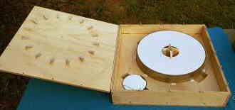 |
I purchased my 16" f/4-f/12 classical Cassegrain mirror set from Scope City, Parks Optical's largest distributor. After I received them, I designed and built a special, secure storage/carrying case for them. Visit Scope City
© 2000 David Anthony Harbour
Contact Dave Harbour via E-mail
(Please contact Bob May if this address goes bad)
| Go to Another place | |
|---|---|
| Previous Page | Start Page |